TransVLM: A Vision-Language Framework and Benchmark for Detecting Any Shot Transitions

Abstract

Traditional Shot Boundary Detection (SBD) inherently struggles with complex transitions by formulating the task around isolated cut points, frequently yielding corrupted video shots. We address this fundamental limitation by formalizing the Shot Transition Detection (STD) task. Rather than searching for ambiguous points, STD explicitly detects the continuous temporal segments of transitions. To tackle this, we propose TransVLM, a Vision-Language Model (VLM) framework for STD. Unlike regular VLMs that predominantly rely on spatial semantics and struggle with fine-grained inter-shot dynamics, our method explicitly injects optical flow as a critical motion prior at the input stage. Through a simple yet effective feature-fusion strategy, TransVLM directly processes concatenated color and motion representations, significantly enhancing its temporal awareness without incurring any additional visual token overhead on the language backbone. To overcome the severe class imbalance in public data, we design a scalable data engine to synthesize diverse transition videos for robust training, alongside a comprehensive benchmark for STD. Extensive experiments demonstrate that TransVLM achieves superior overall performance, outperforming traditional heuristic methods, specialized spatiotemporal networks, and top-tier VLMs.

Framework

Overview of the TransVLM framework. Our framework comprises three core components. (a) Model Architecture: we explicitly inject optical flow as a motion prior via a parameter-efficient strategy. By exclusively expanding the input projection weights of the Vision Patch Embed Layer, the model directly processes concatenated frames of color and optical flow. Crucially, this extracts joint appearance-motion representations without inflating the visual token sequence length, thereby incurring zero additional computational burden on the language model. (b) Data Synthesis: given an arbitrary sequence of clean shots, our scalable data engine automatically synthesizes videos with diverse transitions, simultaneously generating precisely aligned segment-level JSON labels for model training. (c) Arbitrary Video Inference: a temporal sliding-window strategy partitions the input stream into overlapping segments to generate local predictions, which are subsequently aggregated into a continuous global prediction via temporal Non-Maximum Suppression (NMS).

STD Benchmark

Unlike SBD datasets that provide ambiguous shot boundaries, our benchmark re-annotates six public datasets and combines them with synthesized videos to build a comprehensive STD benchmark of 5,215 videos (~100.3 hours, 45,239 transitions), evaluating diverse transition types. All transitions are equipped with segment-level ground-truth labels. We categorize transitions by duration: Cut (<0.1s), Normal (≤1s), and Long (>1s).

Dataset	Domain	Original Label	Total Videos		Total Transitions		Transition Types
Dataset	Domain	Original Label	Count	Dur. (h)	Count	Dur. (s)	Cut	Normal	Long
RAI [3]	TV Shows	Point	10	1.64	1,036	304.4	757	188	91
BBC [4]	Documentaries	Point	11	9.00	4,943	703.7	4,255	582	106
AutoShot (Test) [1]	Short Videos	Point	200	2.01	2,065	545.0	1,008	1,004	53
ClipShots (Test) [5]	Web Videos	Point	500	32.85	6,923	1,548.1	4,798	1,830	295
MovieShots2 (Test) [6]	Movies	Point	282	20.72	14,767	9,566.4	13,436	710	621
SportsShot (Val) [7]	Sports	Point	240	9.37	5,045	944.4	3,899	1,064	82
STD Synthesis Data	Web Videos	Segment	3,972	24.67	10,460	18,249.3	3,593	1,615	5,252
STD Benchmark	Diverse	Segment	5,215	100.26	45,239	31,861.3	31,746	6,993	6,500

Comparison with Baselines

Evaluation Metrics

We propose a rigorous evaluation suite comprising both segment-level and frame-level metrics, parameterized by a temporal tolerance τ (0.0 – 0.5 s) to handle annotator subjectivity at gradual transition boundaries: Segment F₁ (instance retrieval), Frame F₁ (temporal coverage), Absolute Boundary Error (ABE) in seconds, and Real-Time Factor (RTF) for inference efficiency.

Quantitative Comparison

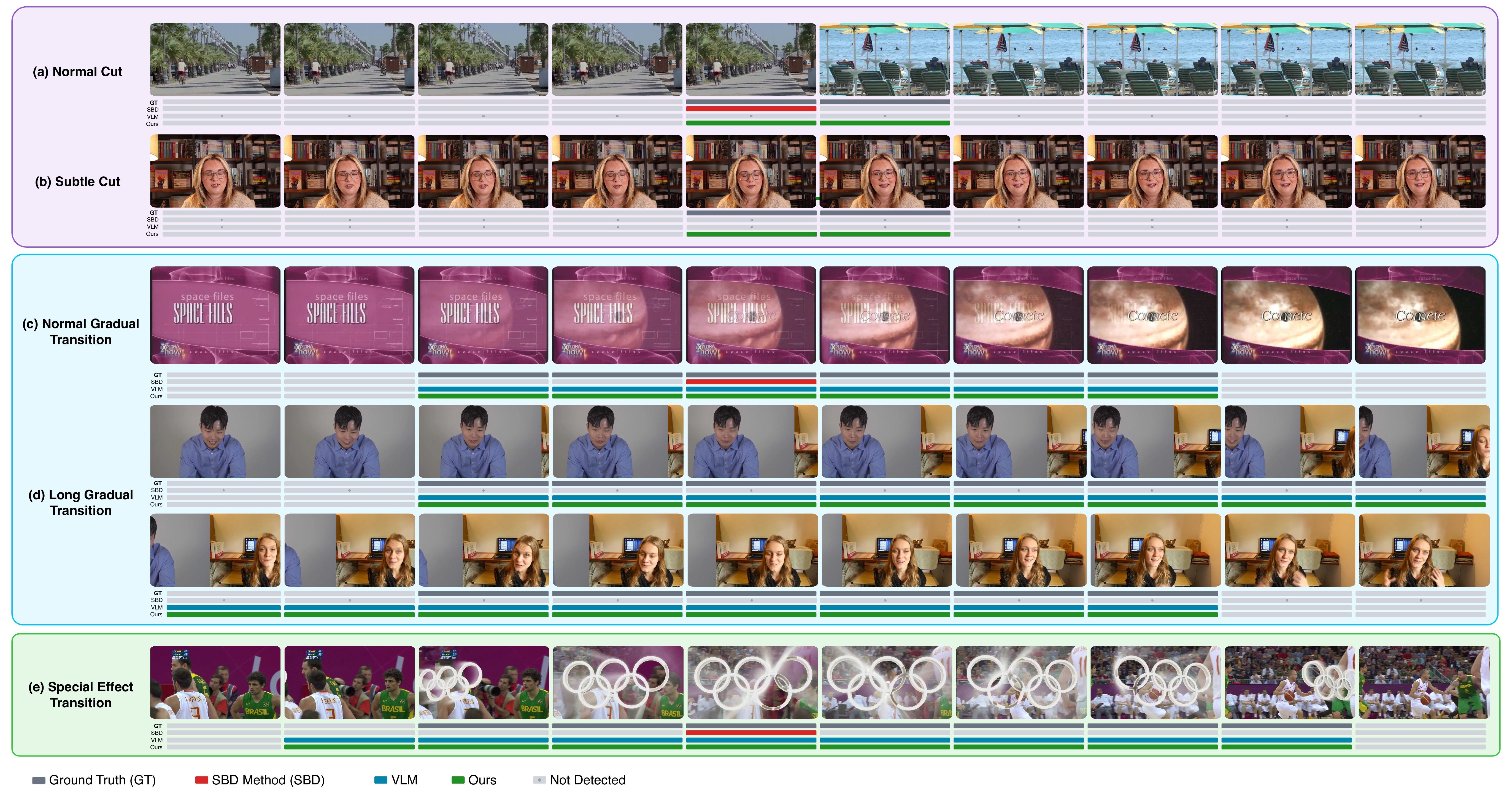
We compare TransVLM against five paradigms: PySceneDetect [8], TransNetV2 [9], AutoShot [1], Gemini series [10], and Qwen3-VL series [2]. We report mean segment- and frame-level metrics across the defined τ values. TransVLM substantially outperforms heuristic methods, specialized networks, and significantly larger general-purpose VLMs. Bold = best, underline = second-best.

Method	Public Data							Synthetic Data							RTF
	Segment			Frame			ABE	Segment			Frame			ABE
	P	R	F₁	P	R	F₁	ABE	P	R	F₁	P	R	F₁	ABE
PySceneDetect [8]
Adaptive	0.656	0.716	0.684	0.645	0.372	0.457	1.93	0.924	0.172	0.290	0.922	0.036	0.069	0.28	0.09
Content	0.627	0.759	0.686	0.603	0.383	0.453	1.08	0.909	0.128	0.225	0.968	0.029	0.056	0.61	0.09
Hash	0.566	0.778	0.654	0.549	0.416	0.457	2.11	0.880	0.118	0.208	0.940	0.027	0.052	0.85	0.09
Hist	0.452	0.741	0.559	0.419	0.398	0.394	1.19	0.577	0.379	0.455	0.762	0.117	0.197	1.04	0.09
Threshold	0.364	0.031	0.057	0.306	0.014	0.027	3.08	0.773	0.039	0.074	0.749	0.008	0.016	1.46	0.09
TransNetV2 [9]	0.727	0.780	0.752	0.731	0.427	0.528	1.87	0.275	0.149	0.194	0.417	0.034	0.063	0.61	0.07
AutoShot [1]	0.707	0.804	0.751	0.709	0.440	0.532	1.78	0.379	0.248	0.299	0.530	0.058	0.102	0.51	0.03
Gemini Series [10]
2.5 Pro	0.558	0.527	0.542	0.453	0.361	0.401	3.62	0.338	0.851	0.465	0.638	0.760	0.686	0.82	0.81
3 Pro	0.527	0.573	0.549	0.469	0.343	0.393	2.18	0.479	0.768	0.588	0.711	0.482	0.568	0.88	1.32
Qwen3-VL Instruct Series [2]
4B	0.235	0.088	0.124	0.134	0.174	0.148	55.00	0.717	0.306	0.428	0.458	0.618	0.525	8.88	0.31
8B	0.222	0.297	0.246	0.132	0.307	0.184	34.39	0.586	0.597	0.591	0.741	0.204	0.315	1.60	0.34
32B	0.309	0.473	0.370	0.214	0.279	0.241	3.96	0.895	0.623	0.735	0.911	0.361	0.516	1.35	0.98
30B-A3B (MoE)	0.218	0.300	0.242	0.171	0.222	0.192	9.61	0.806	0.593	0.683	0.749	0.355	0.482	1.86	0.35
Qwen3-VL Thinking Series [2]
4B	0.449	0.079	0.134	0.265	0.051	0.086	1.50	0.839	0.218	0.346	0.748	0.087	0.156	1.68	1.03
8B	0.450	0.144	0.217	0.297	0.094	0.143	4.25	0.854	0.389	0.534	0.923	0.147	0.252	1.29	1.31
32B	0.403	0.260	0.315	0.308	0.160	0.209	1.09	0.900	0.608	0.726	0.943	0.323	0.479	1.16	3.30
30B-A3B (MoE)	0.374	0.217	0.275	0.291	0.127	0.175	0.98	0.890	0.610	0.724	0.915	0.331	0.485	1.18	0.92
TransVLM (Ours)	0.762	0.806	0.783	0.574	0.562	0.568	1.58	0.908	0.882	0.895	0.946	0.930	0.938	0.11	0.50

Per-τ Comparison & Curves

Use the panels below to inspect detailed per-method numbers across each dataset / temporal tolerance τ, and visualize the corresponding metric curves as a function of τ. In each per-τ table, bold marks the best result and underline marks the second-best.

References

Zhu et al. AutoShot: A Short Video Dataset and State-of-the-Art Shot Boundary Detection. CVPRW 2023.
Bai et al. Qwen3-VL Technical Report. 2025.
Baraldi et al. A Deep Siamese Network for Scene Detection in Broadcast Videos (RAI dataset). ACM MM 2015.
Baraldi et al. Shot and Scene Detection via Hierarchical Clustering for Re-using Broadcast Video (BBC). CAIP 2015.
Tang et al. Fast Video Shot Transition Localization with Deep Structured Models (ClipShots). ACCV 2018.
Rao et al. A Local-to-Global Approach to Multi-Modal Movie Scene Segmentation (MovieShots). CVPR 2020.
MCG. SportsShot: A Large-Scale Sports Shot Boundary Detection Dataset. 2024.
Castellano et al. PySceneDetect. Open-source software, 2014–.
Soucek and Lokoc. TransNet V2: An Effective Deep Network Architecture for Fast Shot Transition Detection. 2020.
Google DeepMind. Gemini Technical Report. 2023.
Zhang et al. NeuFlow v2: Push High-Efficiency Optical Flow to the Limit. 2024.

TransVLM: A Vision-Language Framework and Benchmark for Detecting Any Shot Transitions

Highlights